Charts#
Data#
Every layer may have some data associated with it. The “data” refers to a table of data where each row contains an observation and each column represents a variable that describes some property of each observation.
Data in this format is sometimes referred to as tidy data, flat data, primary data, atomic data, and unit record data.
You can pass tidy data to Lets-Plot in form of a Pandas Dataframe, a Polars Dataframe or just a dictionary: example.
Aesthetics#
Cookbooks:
Basic Building Blocks#
Points:
points,
jittered points
Lines:
line,
path,
diagonal line,
horizontal line,
vertical line,
segment,
curve,
spoke,
step-function
Tiles:
tiles,
rectangles,
raster plot
Text:
text,
text repel,
label,
label repel
Cookbooks:
- Line vs. path
- Missing values: line, path, area, and ribbon
- Indication of removed records
- Drawing graph edges
- Formatting labels on plots
- Text geoms
- Repelled labels
- Image on map, the 'use_crs' parameter
- Variadic lines in geom_path() and geom_line()
- Spoke geometry
- Curve geometry
- Alternating ribbon fill with disjoint groups
- Customizing line type
- Expanding plot limits with expand_limits()
- Configuring nudge units in position adjustments
Demos:
Discrete#
bar,
pie,
lollipop,
boxplot,
count/sum,
bracket,
bracket between dodged groups
Learn more: Working with Categorical Variables and the as_discrete() Function.
Cookbooks:
- Bar geometry
- Pie chart
- Combining discrete and continuous layers
- Annotation labels
- Brackets with labels
- 'boxplot_outlier' statistics
- Lollipop plot
- Count stat
- Handling an overplotting on a scatter plot: geom_count()/stat_sum()
- Using scales
- Generating color palettes with scale.palette()
- Handling color overflow in brewer palettes
- Viridis colors
- Guide to ordering
Contours#
Cookbooks:
Demos:
Visualization of Distribution#
histogram,
density,
dotplot,
ydotplot,
violin,
sina,
ridgeline,
frequency polygon
Cookbooks:
Stats#
stat_ecdf(),
stat_summary(),
stat_summary_bin()
Cookbooks:
Function#
Cookbooks:
Visualization of Errors#
crossbar,
errorbar,
linerange,
pointrange
Cookbooks:
Smoothing#
Use geom_smooth() to draw a fitted smooth curve and, optionally, its confidence interval.
The layer’s labels parameter allows you to display statistical summaries of the fitted model directly on the plot.
For details on available labels and formatting, see Annotations in Lets-Plot.
Cookbooks:
Bivariate Distribution#
2d bins,
2d hexagonal bins,
2d density,
filled 2d density,
pointdensity
Cookbooks:
Marginal Plots#
See also: Joint Plot, Residual Plot.
Cookbooks:
Time Series#
scale_x_datetime(),
scale_y_datetime(),
scale_x_time(),
scale_y_time()
Lets-Plot handles all temporal data types through a unified “datetime” scale (excluding duration/timedelta types, which are handled by the “time” scale). This is in contrast to R’s ggplot2, which provides separate “date”, “time”, and “datetime” scales.
Use break_width in datetime and duration scales to control the axis break interval using human-readable strings like "3 months" or "2 hours".
Supported temporal data types:
Python
timeobjects (time of day)Python
dateobjectsPython
datetimeobjects (both naive and timezone-aware)NumPy
datetime64objectsPandas
Serieswith timezone informationPolars
Serieswith timezone information
Cookbooks:
- Scale time
- Plotting time series
- break_width parameter in datetime scales
- break_width parameter in time (duration) scales
Demos:
Images#
geom_imshow(),
matrix of images
Cookbooks:
- geom_imshow()
- The 'extent' parameter
- Parameters 'norm', 'vmain', 'vmax' and 'cmap'
- The alpha parameter in geom_imshow()
- NaN values in geom_imshow()
- "Fisher boat": 'geom_imshow()' and 'geom_raster()'
- Custom color palettes in geom_imshow()
- DEM image on map
- Image on map, the 'use_crs' parameter
- Image matrix
Facets#
Cookbooks:
Demos:
Coordinate Systems#
coord_cartesian(),
coord_fixed(),
coord_polar(),
coord_flip(),
coord_map()
Cookbooks:
Positional Scales#
scale_x_discrete(),
scale_y_discrete(),
scale_x_discrete_reversed(),
scale_y_discrete_reversed(),
scale_x_continuous(),
scale_y_continuous(),
scale_x_log10(),
scale_y_log10(),
scale_x_log2(),
scale_y_log2(),
scale_x_reverse(),
scale_y_reverse()
Cookbooks:
- Axis position
- break_width parameter in position scales
- Formatting labels on plots
- Zooming map geometry with Lets-Plot
Demos:
Legends and Guides#
guide_legend(),
guide_colorbar(),
guides(),
layer_key()
Cookbooks:
‘bistro’ Plots#
corr_plot(),
qq_plot(),
joint_plot(),
residual_plot(),
waterfall_plot()
“Bistro” plots is a collection of “compound plots” allowing users to generate intricate charts without the need for extensive coding.
With these high-level functions you can create visualizations like correlation matrices, quantile-quantile plots, and joint distribution plots using single function calls.
Learn more: ‘bistro’ Plots.
GeoPandas Shapes#
GeoPandas GeoDataFrame is supported by the following geometry layers: polygon, map, point, pointdensity, pie, text, label, path, rect.
Learn more: GeoPandas Support.
Cookbooks:
Demos:
Grouping Plots#
ggbunch, gggrid and ggdeck shows a collection of plots on one figure.
Cookbooks:
- The ggbunch function
- The gggrid() function
- Dual-axis effect with ggdeck()
- Plot overlay with ggdeck()
- Sharing X,Y-axis scale limits
- Interactive pan/zoom with shared axes in gggrid
- Collecting guides in gggrid()
Demos:
Presentation Options#
theme(),
ggtitle(),
ggsize(),
xlab(),
ylab(),
labs()
Cookbooks:
- Custom theme
- Named system colors
- Tooltip customization
- Customizing fonts
- Axis position
- Rotation of axis labels
- Exponent format in Lets-Plot
- Annotation labels
Predefined Themes#
minimal2,
bw,
grey (or gray),
classic,
light,
minimal,
void,
none


Cookbooks:
Color Schemes (Flavors)#
darcula,
solarized light,
solarized dark,
high contrast light,
high contrast dark,
standard

Cookbooks:
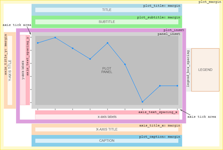
Plot Layout Diagrams#
These diagrams illustrate layout options and their spatial relationships within plot components.
Option names on the diagrams (e.g., axis_text_spacing_x) correspond to theme() function arguments.
Simple options accept numeric values directly, e.g. theme(axis_text_spacing_x=10).
Composite options shown as axis_title_x: margin accept element_text() or element_rect() function results, e.g. theme(axis_title_x=element_text(margin=[5, 5])).
Plot Panel Layout#
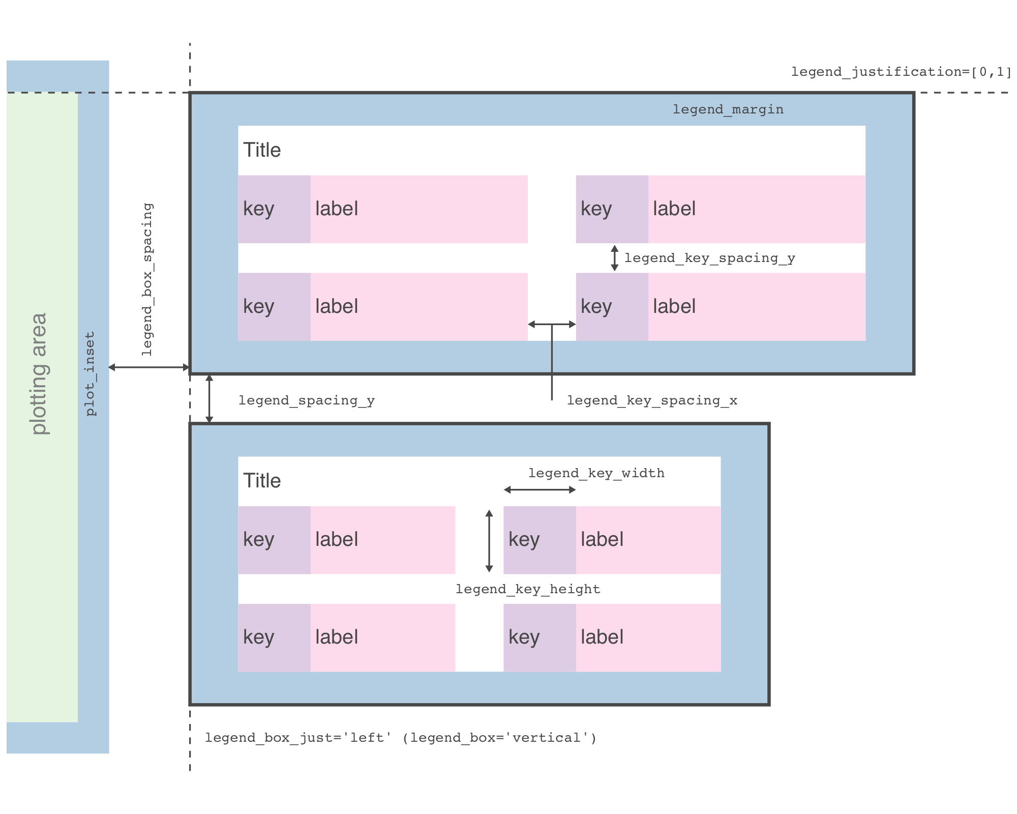
Legend Box Layout#
Miscellaneous#
Panning and Zooming#
Use the ggtb() function to enable Pan and Zoom interactivity on a chart.
This function adds a toolbar containing three tool-buttons: pan, rubber-band zoom, and center-point zoom.
Demos:
Extended Text Markup#
In tooltips/labels/texts and wherever else there is text, you can use:
Interactive links, e.g.
<a href="https://github.com">GitHub</a>.Limited LaTeX support:
superscript, e.g.
\( a^b \),subscript, e.g.
\( x_i \),Greek letters, e.g.
\( \Omega \), andsome special symbols, e.g.
\( a \cdot b \neq c \).
Learn more: LaTeX Support.
Limited markdown support:
emphasis (
*,**,***,_,__,___),coloring with inline style (
<span style='color:red'>text</span>),links with anchor tags (
<a href="https://lets-plot.org">Lets-Plot</a>), andmultiple lines using double space and a newline delimiter (
\n).
Cookbooks:
Demos:
Manual Legend#
In Lets-Plot, as in ggplot2, legends are automatically generated based on the aesthetic mappings in the plot.
Sometimes, however, this automatic generation doesn’t provide the precise control needed for complex visualizations.
Options manual_key and override_aes addresses this limitation.
Cookbooks:
Demos:
Multiple Color Scales#
Use color_by/fill_by parameters and paint_a/paint_b/paint_c aesthetics if you need to display two different layers with the same color aesthetic but different color scales.
Cookbooks:
- Multiple color scales
Waterfall plot, section “Additional Layers with
background_layersParameter”
Demos:
Scale Functions#
To specify a scale for any group of aesthetics, use the special scale functions: scale_manual(), scale_continuous(), scale_gradient(), etc.
Cookbooks:
Demos:
Quantiles#
Density-like plots let you show the quantiles by mapping them to a particular colour palette.
Cookbooks:
Stackable Position Adjustments#
To configure positioning where groups are stacked on top of each other, use the position_stack() and position_fill() functions.
Cookbooks:
Demos:
Resources#
Coding for Economists by Arthur Turrell
Easy Data Visualisation for Tidy Data with Lets-Plot - how to make plots quickly using the declarative plotting.
Python4DS by Arthur Turrell
Data Visualisation - will teach you how to visualise your data using Lets-Plot.
Layers - a deeper dive into aesthetic mappings, geometric objects, and facets.
Exploratory Data Analysis - search for answers by visualising, transforming, and modelling your data.
Data Science with Sanjaya by Sanjaya Subedi
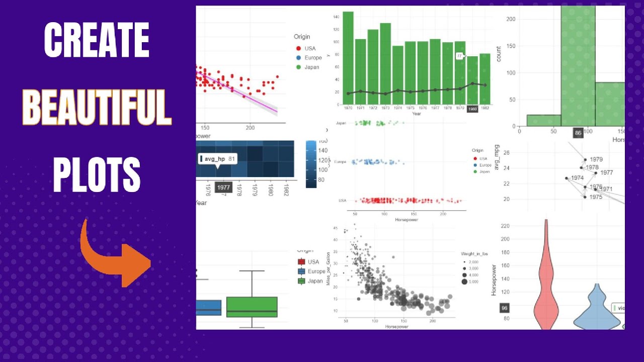
Create Beautiful Plots with Python Let’s Plot Library - Using the Lets-Plot library, the author shows you how to create 10 different but very common types of plots that you’ll see and create often.
Key Features#
Inspired by ggplot2
A faithful port of R’s ggplot2 to Python.
You can learn R’s ggplot2 and the grammar of graphics in the “ggplot2: Elegant Graphics for Data Analysis” book by Hadley Wickham.

Multiplatform
A Grammar of Graphics for Python - works in Python notebooks (Jupyter, Datalore, Kaggle, Colab, Deepnote, Nextjournal) as well as in PyCharm and Intellij IDEA IDEs.
A Grammar of Graphics for Kotlin - a Kotlin multiplatform visualization library which fulfills your needs in the Kotlin ecosystem: from Kotlin notebooks to Compose-Multiplatform apps.


Interactive Maps
Interactive maps allow zooming and panning around your geospatial data with customizable vector or raster basemaps as a backdrop. Learn more.


‘bistro’ Plots
Ready-to-use compound plots - correlation matrices, Q-Q plots, joint plots, residual plots - that combine multiple geoms, scales, and settings into one call. Learn more.


Panning and Zooming
Enable an interactive toolbar with ggtb() to pan and zoom any chart - rubber-band zoom, center-point zoom, and pan tools. Learn more.


Customizable Tooltips and Annotations
You can customize the content, values formatting and appearance of tooltip and annotation for layers of your plot.


Formatting
Lets-Plot supports formatting of numeric and date-time values in tooltips, annotations, legends, on the axes and text geometry layer. Learn more.


Option to Display Plots in External Browser
With the “show externally” mode enabled, you can easily display a plot in an external browser by invoking its show() method. Learn more.


Sampling
Sampling is a special technique of data transformation, which helps to deal with large datasets and overplotting. Learn more.


‘No Javascript’ and Offline Mode
In the ‘no javascript’ mode Lets-Plot generates plots as bare-bones SVG images. Plots in the notebook with option offline=True will be working without an Internet connection. Learn more.