Lets-Plot Cheatbook

Preparation

Imports

from io import BytesIO
import requests

import numpy as np
import pandas as pd
from PIL import Image
from scipy.stats import multivariate_normal

from lets_plot import *
from lets_plot.bistro import *
from lets_plot.geo_data import *

The geodata is provided by © OpenStreetMap contributors and is made available here under the Open Database License (ODbL).

LetsPlot.setup_html()

Data

mpg_df = pd.read_csv('https://raw.githubusercontent.com/JetBrains/lets-plot-docs/master/data/mpg.csv')
mpg_df.head(3)

	Unnamed: 0	manufacturer	model	displ	year	cyl	trans	drv	cty	hwy	fl	class
0	1	audi	a4	1.8	1999	4	auto(l5)	f	18	29	p	compact
1	2	audi	a4	1.8	1999	4	manual(m5)	f	21	29	p	compact
2	3	audi	a4	2.0	2008	4	manual(m6)	f	20	31	p	compact

class_df = mpg_df.groupby('class').hwy.agg(['min', 'median', 'max', 'count']).reset_index()
class_df.head(3)

	class	min	median	max	count
0	2seater	23	25.0	26	5
1	compact	23	27.0	44	47
2	midsize	23	27.0	32	41

fl_df = mpg_df.groupby(['cty', 'hwy']).fl.agg(pd.Series.mode).to_frame('fl').reset_index()
fl_df.head(3)

	cty	hwy	fl
0	9	12	e
1	11	14	[e, p]
2	11	15	r

economics_df = pd.read_csv('https://raw.githubusercontent.com/JetBrains/lets-plot-docs/master/data/economics.csv', parse_dates=['date'])
economics_df.head(3)

	Unnamed: 0	date	pce	pop	psavert	uempmed	unemploy
0	1	1967-07-01	506.7	198712.0	12.6	4.5	2944
1	2	1967-08-01	509.8	198911.0	12.6	4.7	2945
2	3	1967-09-01	515.6	199113.0	11.9	4.6	2958

midwest_df = pd.read_csv('https://raw.githubusercontent.com/JetBrains/lets-plot-docs/master/data/midwest.csv')
midwest_df.head()

	Unnamed: 0	PID	county	state	area	poptotal	popdensity	popwhite	popblack	popamerindian	...	percollege	percprof	poppovertyknown	percpovertyknown	percbelowpoverty	percchildbelowpovert	percadultpoverty	percelderlypoverty	inmetro	category
0	1	561	ADAMS	IL	0.052	66090	1270.961540	63917	1702	98	...	19.631392	4.355859	63628	96.274777	13.151443	18.011717	11.009776	12.443812	0	AAR
1	2	562	ALEXANDER	IL	0.014	10626	759.000000	7054	3496	19	...	11.243308	2.870315	10529	99.087145	32.244278	45.826514	27.385647	25.228976	0	LHR
2	3	563	BOND	IL	0.022	14991	681.409091	14477	429	35	...	17.033819	4.488572	14235	94.956974	12.068844	14.036061	10.852090	12.697410	0	AAR
3	4	564	BOONE	IL	0.017	30806	1812.117650	29344	127	46	...	17.278954	4.197800	30337	98.477569	7.209019	11.179536	5.536013	6.217047	1	ALU
4	5	565	BROWN	IL	0.018	5836	324.222222	5264	547	14	...	14.475999	3.367680	4815	82.505140	13.520249	13.022889	11.143211	19.200000	0	AAR

5 rows × 29 columns

pop_df = midwest_df.groupby('state').poptotal.sum().to_frame('population').reset_index()
pop_df.head(3)

	state	population
0	IL	11430602
1	IN	5544159
2	MI	9295297

states_df = geocode('state', pop_df.state, scope='US').get_boundaries(9)
states_df.head(3)

	state	found name	geometry
0	IL	Illinois	MULTIPOLYGON (((-89.13301 36.98200, -89.16777 ...
1	IN	Indiana	MULTIPOLYGON (((-84.81993 39.10544, -84.83405 ...
2	MI	Michigan	MULTIPOLYGON (((-90.41862 46.56636, -90.00014 ...

def generate_random_data(size=50, mean=[0, 0], cov=[[1, .5], [.5, 1]], seed=42):
    np.random.seed(seed)
    x = np.linspace(-1, 1, size)
    y = np.linspace(-1, 1, size)
    X, Y = np.meshgrid(x, y)
    Z = multivariate_normal(mean, cov).pdf(np.dstack((X, Y)))
    return pd.DataFrame({'x': X.flatten(), 'y': Y.flatten(), 'z': Z.flatten()})

random_df = generate_random_data()
random_df.head(3)

	x	y	z
0	-1.000000	-1.0	0.094354
1	-0.959184	-1.0	0.096849
2	-0.918367	-1.0	0.099189

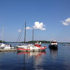
response = requests.get('https://raw.githubusercontent.com/JetBrains/lets-plot-docs/master/source/examples/cookbook/images/fisher_boat.png')
img = Image.open(BytesIO(response.content))
img

Basics

ggplot(mpg_df, aes('cty', 'hwy')) + \
    geom_point(aes(color='cyl')) + \
    geom_smooth(method='lm') + \
    scale_color_brewer(type='div', palette='Spectral') + \
    theme_classic() + \
    ggtitle("Simple linear smoothing")

Features

Interactive Maps

ggplot() + \
    geom_livemap() + \
    geom_map(aes(color='population', fill='population'), \
             data=pop_df, map=states_df, map_join='state', size=1, alpha=.3,
             tooltips=layer_tooltips().format('population', '.3~s')) + \
    scale_color_gradient(low='#1a9641', high='#d7191c', format='.3~s') + \
    scale_fill_gradient(low='#1a9641', high='#d7191c', format='.3~s')

Interactive Plots

ggplot(mpg_df, aes(x='hwy', fill='drv')) + \
    geom_density(alpha=.5) + \
    ggtb()

Customizable Tooltips

ggplot(mpg_df, aes(x='fl', fill=as_discrete('year'))) + \
    geom_bar(tooltips=layer_tooltips().line('fl|^x')
                                      .format('@year', 'd').line('@|@year')
                                      .line('count|@..count..')) + \
    scale_fill_discrete(format="d")

Formatting

ggplot(economics_df, aes('date', 'unemploy')) + \
    geom_area(color='#253494', fill='#41b6c4') + \
    scale_x_datetime(format='%e %b %Y')

Sampling

ggplot(mpg_df, aes('cty', 'hwy')) + \
    geom_point(aes(color=as_discrete('cyl')), sampling=sampling_group_random(2, seed=42))

Images

ggplot() + \
    geom_imshow(np.asarray(img)) + \
    theme_void()

Correlation Plot

corr_plot(data=mpg_df.select_dtypes(include=np.number), threshold=.5)\
    .points().labels()\
    .palette_gradient(low='#d7191c', mid='#ffffbf', high='#1a9641')\
    .build() + \
    ggsize(400, 400)

Joint Plot

joint_plot(data=mpg_df, x='cty', y='hwy')

Residual Plot

residual_plot(data=mpg_df, x='cty', y='hwy', size=5, alpha=.5, color_by='drv', marginal="dens:tr")

Waterfall Plot

waterfall_plot(class_df, "class", "count")

Geoms

Graphical Primitives

ggplot(economics_df, aes('date', 'unemploy')) + scale_x_datetime() + \
    geom_path()

ggplot() + \
    geom_polygon(data=states_df)

ggplot() + \
    geom_rect(xmin=0, xmax=1, ymin=0, ymax=1)

ggplot(economics_df, aes('date', 'unemploy')) + scale_x_datetime() + \
    geom_ribbon(aes(ymin=economics_df.unemploy - 900, ymax=economics_df.unemploy + 900))

ggplot() + \
    geom_band(xmin=-1, xmax=1)

Line Segments

ggplot() + \
    geom_abline(slope=.5)

ggplot() + \
    geom_hline(yintercept=0)

ggplot() + \
    geom_vline(xintercept=0)

ggplot() + \
    geom_segment(x=0, y=0, xend=1, yend=1, arrow=arrow())

ggplot() + \
    geom_curve(x=0, y=0, xend=1, yend=1, curvature=0.3, arrow=arrow())

ggplot() + \
    geom_spoke(x=0, y=0, angle=0.64, radius=5)

One Variable 1

Continuous

ggplot(mpg_df, aes(x='hwy')) + \
    geom_area(stat='bin')

ggplot(mpg_df, aes(x='hwy')) + \
    geom_density()

ggplot(mpg_df, aes(x='hwy')) + \
    geom_freqpoly()

ggplot(mpg_df, aes(x='hwy')) + \
    geom_histogram()

ggplot(mpg_df, aes(x='hwy')) + \
    geom_dotplot(stackratio=.5)

ggplot(mpg_df, aes(sample='hwy')) + \
    geom_qq() + \
    geom_qq_line()

Discrete

ggplot(mpg_df, aes(x='fl')) + \
    geom_bar()

ggplot(mpg_df) + \
    geom_pie(aes(fill='fl'))

ggplot() + \
    geom_function(aes(x='hwy'), data=mpg_df, fun=lambda t: t**.5)

Two Variables 1

Both Continuous

ggplot(mpg_df, aes('cty', 'hwy')) + \
    geom_point()

ggplot(mpg_df, aes('cty', 'hwy')) + \
    geom_smooth()

ggplot(mpg_df, aes('cty', 'hwy')) + \
    geom_qq2() + \
    geom_qq2_line()

ggplot(fl_df, aes('cty', 'hwy')) + \
    geom_text(aes(label='fl'))

ggplot(fl_df, aes('cty', 'hwy')) + \
    geom_point(color="red", size=2) + \
    geom_text_repel(aes(label='fl'), seed=42)

ggplot(fl_df, aes('cty', 'hwy')) + \
    geom_label(aes(label='fl'))

ggplot(fl_df, aes('cty', 'hwy')) + \
    geom_point(color="red", size=2) + \
    geom_label_repel(aes(label='fl'), seed=42)

One Discrete, One Continuous

ggplot(mpg_df, aes('class', 'hwy')) + \
    geom_boxplot()

ggplot(mpg_df, aes('hwy', 'class')) + \
    geom_area_ridges()

ggplot(mpg_df, aes('class', 'hwy')) + \
    geom_violin()

ggplot(mpg_df, aes('class', 'hwy')) + \
    geom_sina(seed=42)

ggplot(mpg_df, aes('class', 'hwy')) + \
    geom_ydotplot(stackratio=.5)

ggplot(class_df, aes('class', 'count')) + \
    geom_bar(stat='identity')

Both Discrete

ggplot(mpg_df, aes('fl', 'drv')) + \
    geom_count()

ggplot(mpg_df, aes('fl', 'drv')) + \
    geom_jitter(seed=42)

Continuous Bivariate Distribution

ggplot(mpg_df, aes('cty', 'hwy')) + \
    geom_bin2d()

ggplot(mpg_df, aes('cty', 'hwy')) + \
    geom_hex()

ggplot(mpg_df, aes('cty', 'hwy')) + \
    geom_density2d(aes(color='..group..'))

ggplot(mpg_df, aes('cty', 'hwy')) + \
    geom_density2df(aes(fill='..group..'))

ggplot(mpg_df, aes('cty', 'hwy')) + \
    geom_pointdensity()

Continuous Function

ggplot(economics_df, aes('date', 'unemploy')) + scale_x_datetime() + \
    geom_area()

ggplot(economics_df, aes('date', 'unemploy')) + scale_x_datetime() + \
    geom_line()

ggplot(economics_df, aes('date', 'unemploy')) + scale_x_datetime() + \
    geom_step()

Visualizing Error

ggplot(class_df, aes(x='class')) + \
    geom_crossbar(aes(ymin='min', y='median', ymax='max'))

ggplot(class_df, aes(x='class')) + \
    geom_errorbar(aes(ymin='min', ymax='max'))

ggplot(class_df, aes(x='class')) + \
    geom_linerange(aes(ymin='min', ymax='max'))

ggplot(class_df, aes(x='class')) + \
    geom_pointrange(aes(ymin='min', y='median', ymax='max'))

Maps

ggplot() + \
    geom_map(data=states_df)

Three Variables 1

ggplot(random_df, aes('x', 'y')) + \
    geom_contour(aes(z='z'))

ggplot(random_df, aes('x', 'y')) + \
    geom_contourf(aes(z='z'), color='white')

ggplot(random_df, aes('x', 'y')) + \
    geom_raster(aes(fill='z'))

ggplot(random_df, aes('x', 'y')) + \
    geom_tile(aes(fill='z'))

Empty Geometry

ggplot() + geom_blank()

Stats

Identity

p_bunch_1 = ggplot(mpg_df, aes('class', 'hwy')) + \
    geom_bar() + \
    ggtitle("Bar geom, default stat")
p_bunch_2 = ggplot(class_df, aes('class', 'count')) + \
    geom_bar(stat='identity') + \
    ggtitle("Bar geom, identity stat")

gggrid([p_bunch_1, p_bunch_2])

One Variable 2

Continuous

ggplot(mpg_df, aes(x='hwy')) + \
    stat_ecdf()

p_bunch_1 = ggplot(mpg_df, aes(x='hwy')) + \
    geom_histogram() + \
    ggtitle("Histogram geom, default stat")
p_bunch_2 = ggplot(mpg_df, aes(x='hwy')) + \
    geom_step(aes(y='..count..'), stat='bin') + \
    ggtitle("Step geom, bin stat")

gggrid([p_bunch_1, p_bunch_2])

p_bunch_1 = ggplot(mpg_df, aes(x='hwy')) + \
    geom_density() + \
    ggtitle("Density geom, default stat")
p_bunch_2 = ggplot(mpg_df, aes(x='hwy')) + \
    geom_point(stat='density') + \
    ggtitle("Point geom, density stat")

gggrid([p_bunch_1, p_bunch_2])

Discrete

p_bunch_1 = ggplot(mpg_df, aes(x='fl')) + \
    geom_bar() + \
    ggtitle("Bar geom, default stat")
p_bunch_2 = ggplot(mpg_df, aes(x='fl')) + \
    geom_lollipop(aes(y='..count..'), stat='count') + \
    ggtitle("Lollipop geom, count stat")

gggrid([p_bunch_1, p_bunch_2])

Two Variables 2

Both Continuous

ggplot(mpg_df, aes('cty', 'hwy')) + \
    stat_summary_bin()

p_bunch_1 = ggplot(mpg_df, aes('cty', 'hwy')) + \
    geom_smooth() + \
    ggtitle("Smooth geom, default stat")
p_bunch_2 = ggplot(mpg_df, aes('cty', 'hwy')) + \
    geom_crossbar(aes(y='hwy', ymin='..ymin..', ymax='..ymax..'), stat='smooth') + \
    ggtitle("Crossbar geom, smooth stat")

gggrid([p_bunch_1, p_bunch_2])

One Discrete, One Continuous

ggplot(mpg_df, aes('class', 'hwy')) + \
    stat_summary()

p_bunch_1 = ggplot(mpg_df, aes('class', 'hwy')) + \
    geom_boxplot() + \
    ylim(10, 50) + \
    ggtitle("Boxplot geom, default stat")
p_bunch_2 = ggplot(mpg_df, aes('class', 'hwy')) + \
    geom_linerange(aes(ymin='..ymin..', ymax='..ymax..'), stat='boxplot', color='black') + \
    geom_errorbar(aes(ymin='..lower..', ymax='..upper..'), stat='boxplot', width=.9) + \
    ylim(10, 50) + \
    ggtitle("Linerange and errorbar geoms, boxplot stat")

gggrid([p_bunch_1, p_bunch_2])

Both Discrete

ggplot(mpg_df, aes('fl', 'drv')) + \
    stat_sum()

Continuous Bivariate Distribution

p_bunch_1 = ggplot(mpg_df, aes('cty', 'hwy')) + \
    geom_bin2d() + \
    ggtitle("Bin2d geom, default stat")
p_bunch_2 = ggplot(mpg_df, aes('cty', 'hwy')) + \
    geom_point(aes(color='..count..'), stat='bin2d') + \
    ggtitle("Point geom, bin2d stat")

gggrid([p_bunch_1, p_bunch_2])

p_bunch_1 = ggplot(mpg_df, aes('cty', 'hwy')) + \
    geom_hex() + \
    ggtitle("Hex geom, default stat")
p_bunch_2 = ggplot(mpg_df, aes('cty', 'hwy')) + \
    geom_point(aes(color='..count..'), stat='binhex') + \
    ggtitle("Point geom, binhex stat")

gggrid([p_bunch_1, p_bunch_2])

p_bunch_1 = ggplot(mpg_df, aes('cty', 'hwy')) + \
    geom_density2d(aes(color='..group..')) + \
    ggtitle("Density2d geom, default stat")
p_bunch_2 = ggplot(mpg_df, aes('cty', 'hwy')) + \
    geom_tile(aes(color='..group..'), stat='density2d', size=.5) + \
    ggtitle("Tile geom, density2d stat")

gggrid([p_bunch_1, p_bunch_2])

Three Variables 2

p_bunch_1 = ggplot(random_df, aes('x', 'y')) + \
    geom_contour(aes(z='z')) + \
    ggtitle("Contour geom, default stat")
p_bunch_2 = ggplot(random_df, aes('x', 'y')) + \
    geom_path(aes(z='z'), stat='contour') + \
    ggtitle("Path geom, contour stat")

gggrid([p_bunch_1, p_bunch_2])

Scales

General Purpose Scales

p_common = ggplot(mpg_df, aes(x='fl')) + \
    geom_bar(aes(fill='fl'))
p_bunch_1 = p_common + \
    ggtitle("Bar geom, default fill scale")
p_bunch_2 = p_common + \
    scale_fill_continuous() + \
    ggtitle("Bar geom, continuous fill scale")

gggrid([p_bunch_1, p_bunch_2])

p_common = ggplot(mpg_df, aes(x='hwy')) + \
    geom_histogram(aes(fill='hwy'))
p_bunch_1 = p_common + \
    ggtitle("Histogram geom, default fill scale")
p_bunch_2 = p_common + \
    scale_fill_discrete(guide='none') + \
    ggtitle("Histogram geom, discrete fill scale")

gggrid([p_bunch_1, p_bunch_2])

p_common = ggplot(mpg_df, aes(x='fl')) + \
    geom_bar(aes(alpha='fl'), color='#0c2c84', fill='#0c2c84')
p_bunch_1 = p_common + \
    ggtitle("Bar geom, default alpha scale")
p_bunch_2 = p_common + \
    scale_alpha_manual(values=[.4, .1, .8, .85, .9]) + \
    ggtitle("Bar geom, manual alpha scale")

gggrid([p_bunch_1, p_bunch_2])

p_common = ggplot(economics_df, aes('date', 'unemploy')) + \
    scale_x_datetime() + \
    geom_point(aes(size='psavert'), shape=21, alpha=.3, show_legend=False)
p_bunch_1 = p_common + \
    ggtitle("Point geom, default size scale")
p_bunch_2 = p_common + \
    scale_size_identity() + \
    ggtitle("Point geom, identity size scale")

gggrid([p_bunch_1, p_bunch_2])

X & Y Location Scales

breaks = [economics_df.date.min(), economics_df.date.median(), economics_df.date.max()]
labels = [str(date).split('-')[0] for date in breaks]
p_common = ggplot(economics_df, aes('date', 'pce')) + geom_line()
p_bunch_1 = p_common + \
    ggtitle("Line geom, default x scale")
p_bunch_2 = p_common + \
    scale_x_datetime() + \
    ggtitle("Line geom, datetime x scale")
p_bunch_3 = p_common + \
    scale_x_time(breaks=breaks, labels=labels) + \
    ggtitle("Line geom, time x scale")

gggrid([p_bunch_1, p_bunch_2, p_bunch_3])

p_common = ggplot(midwest_df, aes('state', 'poptotal')) + \
    geom_jitter(aes(color='state'), seed=42) + \
    coord_flip()
p_bunch_1 = p_common + \
    ggtitle("Jitter geom, default y scale")
p_bunch_2 = p_common + \
    scale_y_log10() + \
    ggtitle("Jitter geom, log10 y scale")

gggrid([p_bunch_1, p_bunch_2])

p_common = ggplot(economics_df, aes('date', 'pce')) + \
    geom_line()
p_bunch_1 = p_common + \
    ggtitle("Line geom, default x scale")
p_bunch_2 = p_common + \
    scale_x_reverse() + \
    ggtitle("Line geom, reversed x scale")

gggrid([p_bunch_1, p_bunch_2])

Color & Fill Scales

Continuous

p_common = ggplot(mpg_df, aes(x='hwy')) + \
    geom_histogram(aes(fill='hwy'))
p_bunch_1 = p_common + \
    ggtitle("Histogram geom, default fill scale")
p_bunch_2 = p_common + \
    scale_fill_grey() + \
    ggtitle("Histogram geom, grey fill scale")

gggrid([p_bunch_1, p_bunch_2])

p_common = ggplot(mpg_df, aes(x='hwy')) + \
    geom_histogram(aes(fill='hwy'))
p_bunch_1 = p_common + \
    ggtitle("Histogram geom, default fill scale")
p_bunch_2 = p_common + \
    scale_fill_gradient(low='#006d2c', high='#edf8e9') + \
    ggtitle("Histogram geom, gradient fill scale")

gggrid([p_bunch_1, p_bunch_2])

p_common = ggplot(mpg_df, aes(x='hwy')) + \
    geom_histogram(aes(fill='hwy'))
p_bunch_1 = p_common + \
    ggtitle("Histogram geom, default fill scale")
p_bunch_2 = p_common + \
    scale_fill_brewer(type='seq', palette='GnBu', direction=-1) + \
    ggtitle("Histogram geom, brewer fill scale")

gggrid([p_bunch_1, p_bunch_2])

p_common = ggplot(mpg_df, aes(x='hwy')) + \
    geom_histogram(aes(fill='hwy'))
p_bunch_1 = p_common + \
    ggtitle("Histogram geom, default fill scale")
p_bunch_2 = p_common + \
    scale_fill_viridis(option='inferno') + \
    ggtitle("Histogram geom, viridis fill scale")

gggrid([p_bunch_1, p_bunch_2])

p_common = ggplot(mpg_df, aes(x='hwy')) + \
    geom_histogram(aes(fill='hwy'))
p_bunch_1 = p_common + \
    ggtitle("Histogram geom, default fill scale")
p_bunch_2 = p_common + \
    scale_fill_hue(l=80, c=150) + \
    ggtitle("Histogram geom, hue fill scale")

gggrid([p_bunch_1, p_bunch_2])

p_common = ggplot(random_df, aes('x', 'y')) + \
    geom_histogram(aes(fill='x'), bins=7)
p_bunch_1 = p_common + \
    ggtitle("Histogram geom, default fill scale")
p_bunch_2 = p_common + \
    scale_fill_gradient2(low='#4575b4', mid='#ffffbf', high='#d73027') + \
    ggtitle("Histogram geom, gradient2 fill scale")

gggrid([p_bunch_1, p_bunch_2])

Discrete

p_common = ggplot(mpg_df, aes(x='fl')) + \
    geom_bar(aes(fill='fl'))
p_bunch_1 = p_common + \
    ggtitle("Bar geom, default fill scale")
p_bunch_2 = p_common + \
    scale_fill_brewer(type='qual', palette='Dark2') + \
    ggtitle("Bar geom, brewer fill scale")

gggrid([p_bunch_1, p_bunch_2])

p_common = ggplot(mpg_df, aes(x='fl')) + \
    geom_bar(aes(fill='fl'))
p_bunch_1 = p_common + \
    ggtitle("Bar geom, default fill scale")
p_bunch_2 = p_common + \
    scale_fill_manual(values=['#fbb4ae', '#b3cde3', '#ccebc5', '#decbe4', '#fed9a6']) + \
    ggtitle("Bar geom, manual fill scale")

gggrid([p_bunch_1, p_bunch_2])

Size & Shape Scales

p_common = ggplot(mpg_df, aes('cty', 'hwy')) + \
    geom_point(aes(size='cyl'), shape=21, alpha=.2)
p_bunch_1 = p_common + \
    ggtitle("Point geom, default size scale")
p_bunch_2 = p_common + \
    scale_size_area() + \
    ggtitle("Point geom, area size scale")

gggrid([p_bunch_1, p_bunch_2])

p_common = ggplot(mpg_df, aes('cty', 'hwy')) + \
    geom_point(aes(size='cyl'), shape=21, alpha=.2)
p_bunch_1 = p_common + \
    ggtitle("Point geom, default size scale")
p_bunch_2 = p_common + \
    scale_size(range=[3, 6]) + \
    ggtitle("Point geom, size scale in range 3..6")

gggrid([p_bunch_1, p_bunch_2])

p_common = ggplot(mpg_df[mpg_df["fl"] == "p"], aes('hwy', 'cty')) + \
    geom_lollipop(aes(linewidth='cyl'), slope=.7, intercept=.8, dir='s') + \
    coord_fixed()
p_bunch_1 = p_common + \
    ggtitle("Lollipop geom, default linewidth scale")
p_bunch_2 = p_common + \
    scale_linewidth(range=[.5, 2]) + \
    ggtitle("Lollipop geom, scaled linewidth")

gggrid([p_bunch_1, p_bunch_2])

p_common = ggplot(mpg_df, aes('cty', 'hwy')) + \
    geom_point(aes(stroke='cyl'), shape=1, alpha=.2)
p_bunch_1 = p_common + \
    ggtitle("Point geom, default stroke scale")
p_bunch_2 = p_common + \
    scale_stroke(range=[.5, 2]) + \
    ggtitle("Point geom, scaled stroke")

gggrid([p_bunch_1, p_bunch_2])

p_common = ggplot(fl_df, aes('cty', 'hwy')) + \
    geom_point(aes(shape='fl'))
p_bunch_1 = p_common + \
    ggtitle("Point geom, default shape scale")
p_bunch_2 = p_common + \
    scale_shape(solid=False) + \
    ggtitle("Point geom, shape scale with solid=False")

gggrid([p_bunch_1, p_bunch_2])

p_common = ggplot(fl_df, aes('cty', 'hwy')) + \
    geom_point(aes(shape='fl'))
p_bunch_1 = p_common + \
    ggtitle("Point geom, default shape scale")
p_bunch_2 = p_common + \
    scale_shape_manual(values=[0, 12, 1, 10, 3, 13, 2, 4]) + \
    ggtitle("Point geom, manual shape scale")

gggrid([p_bunch_1, p_bunch_2])

Coordinate Systems

p_common = ggplot(mpg_df, aes(x='fl')) + \
    geom_bar()
p_bunch_1 = p_common + \
    ggtitle("Bar geom, default coordinate system")
p_bunch_2 = p_common + \
    coord_cartesian(ylim=[0, 250]) + \
    ggtitle("Bar geom, cartesian coordinate system")

gggrid([p_bunch_1, p_bunch_2])

p_common = ggplot(mpg_df, aes('cty', 'hwy')) + \
    geom_point()
p_bunch_1 = p_common + \
    ggtitle("Point geom, default coordinate system")
p_bunch_2 = p_common + \
    coord_polar() + \
    ggtitle("Point geom, polar coordinate system")

gggrid([p_bunch_1, p_bunch_2])

p_common = ggplot(mpg_df, aes('cty', 'hwy')) + \
    geom_point()
p_bunch_1 = p_common + \
    ggtitle("Point geom, default coordinate system")
p_bunch_2 = p_common + \
    coord_fixed() + \
    ggtitle("Point geom, fixed coordinate system")

gggrid([p_bunch_1, p_bunch_2])

p_common = ggplot() + \
    geom_polygon(data=states_df)
p_bunch_1 = p_common + \
    ggtitle("Polygon geom, default coordinate system")
p_bunch_2 = p_common + \
    coord_map() + \
    ggtitle("Polygon geom, map coordinate system")

gggrid([p_bunch_1, p_bunch_2])

p_common = ggplot(mpg_df, aes(x='fl')) + \
    geom_bar()
p_bunch_1 = p_common + \
    ggtitle("Bar geom, default coordinate system")
p_bunch_2 = p_common + \
    coord_flip() + \
    ggtitle("Bar geom, flipped coordinates")

gggrid([p_bunch_1, p_bunch_2])

Position Adjustments

p_bunch_1 = ggplot(mpg_df, aes(x='fl')) + \
    geom_bar(aes(fill='drv')) + \
    ggtitle("Bar geom, default position")
p_bunch_2 = ggplot(mpg_df, aes(x='fl')) + \
    geom_bar(aes(fill='drv'), position='dodge') + \
    ggtitle("Bar geom, dodge position")

gggrid([p_bunch_1, p_bunch_2])

p_bunch_1 = ggplot(mpg_df, aes(x='hwy')) + \
    geom_density(aes(fill='drv'), color="black") + \
    ggtitle("Density geom, default position")
p_bunch_2 = ggplot(mpg_df, aes(x='hwy')) + \
    geom_density(aes(fill='drv'), color="black", position='stack') + \
    ggtitle("Density geom, stack position")
p_bunch_3 = ggplot(mpg_df, aes(x='hwy')) + \
    geom_density(aes(fill='drv'), color="black", position='fill') + \
    ggtitle("Density geom, fill position")

gggrid([p_bunch_1, p_bunch_2, p_bunch_3])

p_bunch_1 = ggplot(mpg_df, aes('cty', 'hwy')) + \
    geom_point() + \
    ggtitle("Point geom, default position")
p_bunch_2 = ggplot(mpg_df, aes('cty', 'hwy')) + \
    geom_point(position=position_jitter(seed=42)) + \
    ggtitle("Point geom, jitter position")

gggrid([p_bunch_1, p_bunch_2])

p_common = ggplot(mpg_df, aes('cyl', 'hwy', fill='drv'))
p_bunch_1 = p_common + \
    geom_boxplot() + \
    geom_point(color='black', shape=21) + \
    ggtitle("Point geom, default position")
p_bunch_2 = p_common + \
    geom_boxplot() + \
    geom_point(position=position_jitterdodge(seed=42), \
               color='black', shape=21) + \
    ggtitle("Point geom, jitterdodge position")

gggrid([p_bunch_1, p_bunch_2])

p_common = ggplot(mpg_df, aes('class', 'hwy')) + \
    geom_bar()
p_bunch_1 = p_common + \
    geom_text(aes(label='..count..'), stat='count') + \
    ggtitle("Text geom, default position")
p_bunch_2 = p_common + \
    geom_text(aes(label='..count..'), stat='count', color='white', \
              position=position_nudge(y=-2.5)) + \
    ggtitle("Text geom, nudge position")

gggrid([p_bunch_1, p_bunch_2])

Themes

p_common = ggplot(mpg_df, aes('cty', 'hwy')) + \
    geom_point()
p_bunch = []
p_bunch.append(p_common + ggtitle("Default theme"))
p_bunch.append(p_common + theme_none() + ggtitle("Empty theme"))
p_bunch.append(p_common + theme_void() + ggtitle("Void theme"))
p_bunch.append(p_common + theme_minimal() + ggtitle("Minimalistic theme"))
p_bunch.append(p_common + theme_classic() + ggtitle("Classic theme"))
p_bunch.append(p_common + theme_grey() + ggtitle("Grey theme"))
p_bunch.append(p_common + theme_light() + ggtitle("Light theme"))
p_bunch.append(p_common + theme_bw() + ggtitle("Dark-on-light theme"))

gggrid(p_bunch, ncol=2)

background_color_light = '#ffffe5'
main_color_dark = '#00441b'
main_color_normal = '#238b45'
main_color_light = '#f7fcf5'

custom_theme = theme(
    line=element_line(color=main_color_normal, size=2),
    rect=element_rect(color=main_color_normal, fill=main_color_light, size=2),
    text=element_text(color=main_color_dark, family="Courier", face="bold"),
    geom=element_geom(pen=main_color_normal),
    axis_ontop=True,
    axis_ticks=element_line(color=main_color_normal, size=1),
    axis_ticks_length=7,
    legend_background=element_rect(size=1),
    legend_position='bottom',
    panel_grid_major=element_line(color=main_color_normal, size=.5),
    panel_grid_minor='blank',
    plot_background=element_rect(fill=background_color_light, size=1),
    axis_tooltip=element_rect(color=main_color_dark)
)

ggplot(mpg_df, aes('cty', 'hwy')) + \
    geom_point() + \
    theme_none() + \
    custom_theme + \
    ggtitle("Custom theme")

Flavors

p_common = ggplot(mpg_df, aes('cty', 'hwy')) + \
    geom_point() + \
    theme_grey()
p_bunch = []
p_bunch.append(p_common + ggtitle("Without flavor"))
p_bunch.append(p_common + flavor_darcula() + ggtitle("flavor_darcula()"))
p_bunch.append(p_common + flavor_solarized_light() + ggtitle("flavor_solarized_light()"))
p_bunch.append(p_common + flavor_solarized_dark() + ggtitle("flavor_solarized_dark()"))
p_bunch.append(p_common + flavor_high_contrast_light() + ggtitle("flavor_high_contrast_light()"))
p_bunch.append(p_common + flavor_high_contrast_dark() + ggtitle("flavor_high_contrast_dark()"))

gggrid(p_bunch, ncol=2)

Faceting

ggplot(mpg_df, aes('cty', 'hwy')) + \
    geom_point() + \
    facet_grid(x='fl', y='year', y_format='d')

ggplot(mpg_df, aes('cty', 'hwy')) + \
    geom_point() + \
    facet_wrap(facets='fl', ncol=3)

Labels & Legends

p_common = ggplot(mpg_df, aes('cty', 'hwy')) + \
    geom_point()
p_bunch_1 = p_common + \
    ggtitle("Default plot")
p_bunch_2 = p_common + \
    labs(x='City miles per gallon', y='Highway miles per gallon') + \
    ggtitle("Use labs()")

gggrid([p_bunch_1, p_bunch_2])

p_common = ggplot(mpg_df, aes('cty', 'hwy')) + \
    geom_point()
p_bunch_1 = p_common + \
    ggtitle("Default plot")
p_bunch_2 = p_common + \
    xlab('City miles per gallon') + \
    ylab('Highway miles per gallon') + \
    ggtitle("Use xlab() and ylab()")

gggrid([p_bunch_1, p_bunch_2])

p_common = ggplot(mpg_df, aes(x='fl')) + \
    geom_bar(aes(fill='fl'))
p_bunch_1 = p_common + \
    ggtitle("Default plot")
p_bunch_2 = p_common + \
    theme(legend_position='top') + \
    ggtitle("Use legend_position='top'")

gggrid([p_bunch_1, p_bunch_2])

p_common = ggplot(mpg_df, aes('cty', 'hwy')) + \
    geom_point(aes(color='hwy'))
p_bunch_1 = p_common + \
    ggtitle("Default plot")
p_bunch_2 = p_common + \
    scale_color_gradient(
        guide=guide_colorbar(nbin=40, barwidth=10, barheight=200)
    ) + \
    ggtitle("Use guide_colorbar()")

gggrid([p_bunch_1, p_bunch_2])

p_common = ggplot(mpg_df, aes(x='fl')) + \
    geom_bar(aes(fill='manufacturer')) + \
    theme(legend_position='bottom')
p_bunch_1 = p_common + \
    ggtitle("Default plot")
p_bunch_2 = p_common + \
    scale_fill_discrete(guide=guide_legend(nrow=3)) + \
    ggtitle("Use guide_legend()")

gggrid([p_bunch_1, p_bunch_2])

Zooming

p_common = ggplot() + \
    geom_map(data=states_df) + \
    theme_classic()
p_bunch_1 = p_common + \
    ggtitle("Default plot")
p_bunch_2 = p_common + \
    scale_x_continuous(limits=[-92, -82]) + \
    ylim(36, 43) + \
    ggtitle("Zoom with clipping")
p_bunch_3 = p_common + \
    coord_map(xlim=[-92, -82], ylim=[36, 43]) + \
    ggtitle("Zoom without clipping")

gggrid([p_bunch_1, p_bunch_2, p_bunch_3])